The Kalinga War (ended c. 261 BCE)[1] was fought in ancient India between the Maurya Empire under Ashoka and the state of Kalinga, an independent feudal kingdom located on the east coast, in the present-day state of Odisha and northern parts of Andhra Pradesh. It is presumed that the battle was fought on Dhauli hills in Dhauli which is situated on the banks of Daya River. The Kalinga War was one of the largest and deadliest battles in Indian history.[6]
Kalinga War Part of Conquests of Mauryan Empire
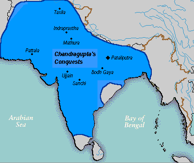
Kalinga (adjacent to the Bay of Bengal) and the Maurya Empire (blue) before the attack of Ashoka The Great Date began c. 262 BCE, ended c. 261 BCE, in the 8th year of Ashoka’s coronation of 268 BCE[1] Location Kalinga, India Result Decisive Mauryan victory Territorial changes Kalinga conquered by Mauryan Empire
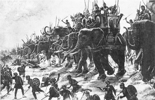
Belligerents Mauryan Empire Kalinga Commanders and leaders Ashoka Unknown Strength Total 600,000[citation needed] 150,000 infantry,[2] 10,000 cavalry[3]
700 war elephants[2] Casualties and losses 70,000[citation needed] 100,000 killed, 150,000 deported (figures by Ashoka)[4][5] This is the only major war Ashoka fought after his accession to the throne, and marked the close of the empire-building and military conquests of ancient India that began with the Mauryan Emperor Chandragupta Maurya.[7] The war cost nearly 250,000 lives.[7]
Kalinga (adjacent to the Bay of Bengal) and the Maurya Empire (blue) before the attack of Ashoka The Great Date began c. 262 BCE, ended c. 261 BCE, in the 8th year of Ashoka’s coronation of 268 BCE[1] Location Kalinga, India Result Decisive Mauryan victory Territorial changes Kalinga conquered by Mauryan Empire
Belligerents Mauryan Empire Kalinga Commanders and leaders Ashoka Unknown Strength Total 600,000[citation needed] 150,000 infantry,[2] 10,000 cavalry[3]
700 war elephants[2] Casualties and losses 70,000[citation needed] 100,000 killed, 150,000 deported (figures by Ashoka)[4][5].
Course of the war
A view of the banks of the Daya River, the supposed battlefield of Kalinga from atop Dhauli hills, Bhubaneswar, Odisha State
No war in the history of India is as important either for its intensity or for its results as the Kalinga war of Ashoka. No wars in the annals of human history have changed the heart of the victor from one of wanton cruelty to that of exemplary piety as this one. From its fathomless womb, the history of the world may find out only a few wars to its credit which may be equal to this war and not a single one that would be greater than this. The political history of mankind is really a history of wars and no war has ended with so successful a mission of peace for the entire war-torn humanity as the war of Kalinga.
Ramesh Prasad Mohapatra, Military History of Odisha
The war was completed in the eighth year of Ashoka’s reign, according to his own Edicts of Ashoka, probably in 261 BCE.[1] After a bloody battle for the throne following the death of his father, Ashoka was successful in conquering Kalinga – but the consequences of the savagery changed Ashoka’s views on war and led him to pledge to never again wage a war of conquest.
According to Megasthenes, the Greek historian at the court of Chandragupta Maurya, the ruler of Kalinga had a powerful army comprising infantry, cavalry and elephants.[13]
Aftermath
Shanti Stupa, Dhauli hill is presumed to be the area where the Kalinga War was fought.
Ashoka had seen the bloodshed and felt that he was the cause of the destruction. The whole area of Kalinga was plundered and destroyed. Some of Ashoka’s later edicts state that about 150,000 people died on the Kalinga side and an almost equal number of Ashoka’s army, though legends among the Odia people – descendants of Kalinga’s natives – claim that these figures were highly exaggerated by Ashoka. As per the legends, Kalinga armies caused twice the amount of destruction they suffered. However, prominent historians have rejected this claim and the edicts of Ashoka are believed to be the primary evidence. Thousands of men and women were deported from Kalinga and forced to work on clearing wastelands for future settlement.[14]
Beloved-of-the-Gods, King Priyadarsi(Ashoka)conquered the Kalingas eight years after his coronation. One hundred and fifty thousand were deported, one hundred thousand were killed and many more died (from other causes). After the Kalingas had been conquered, Beloved-of-the-Gods came to feel a strong inclination towards the Dharma, a love for the Dharma and for instruction in Dharma. Now Beloved-of-the-Gods feels deep remorse for having conquered the Kalingas.
Ashoka, Rock Edict No. 13
Ashoka’s response to the Kalinga War is recorded in the Edicts of Ashoka. The Kalinga War prompted Ashoka, already a non-engaged Buddhist, to devote the rest of his life to ahimsa (non-violence) and to dharma-Vijaya (victory through dharma). Following the conquest of Kalinga, Ashoka ended the military expansion of the empire and began an era of more than 40 years of relative peace, harmony, and prosperity.[citation needed]
References
Le Huu Phuoc, Buddhist Architecture, Grafikol 2009, p.30
Class 12 Economics: Microeconomics – Production and Costs – Get here the Notes for Class 12 Economics: Microeconomics – Production and Costs. Candidates who are ambitious to qualify the Class 12 with good score can check this article for Notes. This is possible only when you have the best CBSE Class 12 Economics Notes,study material, and a smart preparation plan. CBSE 2019 Class 12th Exam is approaching and candidates will have to make the best use of the time available towards the last stage of your CBSE Class 12th Economics Preparation. To help you with that, below we have provided the Notes of 12 Economics for topic Microeconomics – Production and Costs.
Study Materials BYJU’S Answer Scholarship BTC Buy a Course Success Stories Live QuizNEW Login byjus.com Type yo
NCERT SolutionsNCERT Class 12NCERT Class 12 EconomicsNCERT Class 12 Micro EconomicsChapter 3: Production And Costs Top Banner NCERT Solution for Class 12 Microeconomics Chapter 3 – Production and Costs NCERT Solutions are exceptionally helpful books while preparing for the CBSE Class 12 Economics examinations. These Solutions of NCERT are crafted by the subject matter experts to help students learn the concepts effortlessly and prepare well for the board exam.
Download the PDF of NCERT Solutions for Class 12 Economics Chapter 3
ncert solutions for class 12 microeconomics chapter 3 production and costs 15
Previous
Next
Access NCERT Solutions for Class 12 Economics Chapter 3 1. Explain the concept of a production function.
The production function is defined as the relationship between physical inputs used in production and the corresponding physical output. This shows how many units of inputs produce the maximum output. It can be represented as
Qx = f (L, K)
Where Qx = Total Physical Output
L= Total physical labour employed
K= Total capital employed
2. What is the total product of input?
It refers to the total volume of goods and services that are produced in a firm with the provided input during a specific time period.
3. What is the average product of input?
The Average Product of an input is the Total Product divided by the total amount of the variable input used to produce it.
4. What is the marginal product of input?
The marginal product of an input is the improvement in output that is achieved by using an additional unit of input.
5. Explain the relationship between the marginal products and the total product of an input.
This can be explained with the help of the law of variable proportions. As per this law, when only one variable factor input is allowed to increase with all other inputs kept constant, the following changes are observed:
1. With an increase in Marginal Product (MP), there is a corresponding increase in Total Product (TP). A convex curve is obtained with the effect till the MP curve is at its maximum.
2. When MP declines but is positive, then TP increases with a decline in rate, giving the total product a concave shape.
3. When MP is at zero, the TP is at maximum
4. When MP becomes negative, the TP falls.
NCERT Microeconomics Solutions for Class 12 Chapter 3 – 1
6. Explain the concepts of the short run and the long run.
The long run is a period of time in which the producer can change all the variables involved in the production, like building, machine etc. The short-run is a period of time in which the producer can only make limited changes in the production process. It is the period in which at least one factor of production is fixed while others can be changed or improved. The examples of short run can be farmer having a fixed piece of land.
7. What is the law of diminishing marginal product?
According to the law of diminishing marginal product, there will initially be an increase in the total amount of production when one of the factors is increased while keeping the others constant.
Eventually, this strategy would not keep increasing production. For example, think of a factory where the machinery is a factor of production. Increasing the number of machines would initially increase production. But if the company keeps increasing the number of machines without correspondingly hiring new workers to operate them, the productivity will decrease.
8. What is the law of variable proportions?
The Law of Variable Proportions is also called the Law of Diminishing Returns.
According to the law, when one of the inputs involved in the production is changed while keeping the other inputs constant, there will be a point after which the output per unit of that input will start to decrease. This law is theorised under certain assumptions.
i) The technology should remain the same.
ii) The possibility that the factors of production can be changed within a short period of time.
iii) Some inputs should be kept constant
9. When does a production function satisfy constant returns to scale?
Constant returns to scale is achieved when the change in the factors of production matches with the changes in the total output. This means that the efforts of the producer to improve production yield appropriate and equivalent returns.
10. When does a production function satisfy increasing returns to scale?
Increasing returns to scale is achieved when the change in the factors of production yields more than the proportionate changes in the total output. This means that the company has improved its productivity.
11. When does a production function satisfy decreasing returns to scale?
Decreasing returns to scale is when the change in the factors of production results in a decrease in the changes in the total output. This is an indication that the changes have proved to be detrimental to productivity instead of increasing productivity
12. Briefly explain the concept of the cost function.
The relationship between the cost of production and the total output is known as the cost function.
13. What are the total fixed cost, total variable cost and total cost of a firm? How are they related?
A fixed cost is a cost that does not change in relation to the total number of goods and services produced by the company. On the other hand, a variable cost is a cost that changes in relation to the total number of goods and services produced by the company.
Total Fixed Cost: The cost incurred by a company in acquiring fixed production factors like buildings, cost of machinery and depreciation.
Total Variable Cost: Cost incurred by a company on variable production factors like wages and fuel charges.
Total Cost: The total cost of the firm is the total fixed cost and total variable cost put together. It is the actual cost incurred by the company when producing a given amount of output.
14. What are the average fixed cost, average variable cost and average cost of a firm? How are they related?
The average fixed cost is the fixed cost per unit of output produced.
The average variable cost is the variable cost per unit of output produced.
The average cost of a firm is the average fixed cost and average variable cost put together.
15. Can there be some fixed cost in the long run? If not, why?
The fixed cost cannot be set in the long run. Fixed costs can only be set for the short run. Since all factors of production and inputs can change in the long run, a fixed cost cannot be determined for the output.
16. What does the average fixed cost curve look like? Why does it look so?
The average fixed cost resembles a rectangular hyperbola. This is because of the constantly increasing output and the fixed cost, which remains the same at every point.
17. What do the short run marginal cost, average variable cost and short run average cost curves look like?
The curves of the short run marginal cost, the average variable cost and the short run average cost are all U-shaped.
18. Why does the SMC curve cut the AVC curve at the minimum point of the AVC curve?
It can be explained by the following points:
1. When AVC (Average Variable Cost) falls, SMC (Short Marginal Curve) is lesser than AVC.
2. When AVC rises, SMC becomes more than AVC
3. When AVC is constant and is minimum, SMC is equal to AVC.
Therefore, the SMC curve cuts the AVC curve at the minimum point.
19. At which point does the SMC curve intersect SAC curve? Give reasons in support of your answer.
This can be explained with the following points:
1. When SAC falls, SMC is below the SAC.
2. When SAC rises, SMC is above SAC.
Therefore, the SMC curve cuts the SAC curve at its minimum point because at that point, SMC = SAC
20. Why is the short run marginal cost curve ‘U’-shaped?
NCERT Microeconomics Solutions for Class 12 Chapter 3 – 2
The Marginal Curve (MC) is U-shaped as per the Law of Variable Proportion.
This can be explained as follows:
1. Shape of the Marginal Cost Curve (MC) depends on the Total Variable Cost (TVC).
2. As TVC increases at a diminishing rate, the total product increases at an increasing rate, which creates a gap in the curve leading to the fall of MC.
3. Now, as TVC increases at an increasing rate and the total product increases at a diminishing rate, making the marginal cost increase and rise upward.
4. The increasing returns and then constant returns, along with the rise in decreasing returns, make it appear like the letter U from the English alphabet; hence, it is named so.
21. What do the long run marginal cost and the average cost curves look like?
NCERT Microeconomics Solutions for Class 12 Chapter 3 -3
The Long Run Marginal Cost (LMC) and Long Run Average Cost (LAC) are U-shaped, and the reason behind this is the law of returns to scale. As per this law, a company or a firm undergoes three stages in production which are IRS (Increasing Return to Scale), CRS (Constant Return to Scale) and DRS (Diminishing Return to Scale). The curve becomes U-Shaped due to the falling of LAC due to economies of scale (IRS); it attains constant output at the CRS level, and finally, if the firm experiences diseconomies of scale and if it is continuing production after this stage, it will see a rise or DRS.
22. The following table gives the total product schedule of labour. Find the corresponding average product and marginal product schedules of labour.
L TPL 0 0 1 15 2 35 3 50 4 40 5 48 The solution to this question is as follows:
NCERT Microeconomics Solutions for Class 12 Chapter 3 – 4
23. The following table gives the average product schedule of labour. Find the total product and marginal product schedules. It is given that the total product is zero at zero level of labour employment.
L APL 1 2 2 3 3 4 4 4.25 5 4 6 3.5 The solution to this question is as follows:
NCERT Microeconomics Solutions for Class 12 Chapter 3 – 5
24. The following table gives the marginal product schedule of labour. It is also given that the total product of labour is zero at zero level of employment. Calculate the total and average product schedules of labour.
L MPL 1 3 2 5 3 7 4 5 5 3 6 1 The solution to this question is as follows:
NCERT Microeconomics Solutions for Class 12 Chapter 3 – 6
25. The following table shows the total cost schedule of a firm. What is the total fixed cost schedule of this firm?
Calculate the TVC, AFC, AVC, SAC and SMC schedules of the firm.
L TPL 0 10 1 30 2 45 3 55 4 70 5 90 6 120 The solution to this question can be as follows:
NCERT Microeconomics Solutions for Class 12 Chapter 3 – 7
26. The following table gives the total cost schedule of a firm. It is also given that the average fixed cost at 4 units of output is Rs 5/-. Find the TVC, TFC, AVC, AFC, SAC and SMC schedules of the firm for the corresponding values of output.
L TPL 1 50 2 65 3 75 4 95 5 130 6 185 The solution to this question is as follows:
NCERT Microeconomics Solutions for Class 12 Chapter 3- 8
27. A firm’s SMC schedule is shown in the following table. The total fixed cost of the firm is Rs 100. Find the TVC, TC, AVC and SAC schedules of the firm.
L TPL 0 − 1 500 2 300 3 200 4 300 5 500 6 800 The solution to this question is as follows:
NCERT Microeconomics Solutions for Class 12 Chapter 3 – 9
28. Let the production function of a firm beNCERT Microeconomics Solutions for Class 12 Chapter 3 – 10.
Find out the maximum possible output that the firm can produce with 100 units of L and 100 units of K.
The solution is as follows:
NCERT Microeconomics Solutions for Class 12 Chapter 3 -11
29. Let the production function of a firm be Q = 2L2 K2.
Find out the maximum possible output that the firm can produce with 5 units of L and 2 units of K. What is the maximum possible output that the firm can produce with zero unit of L and 10 units of K?
NCERT Microeconomics Solutions for Class 12 Chapter 3 – 12
NCERT Microeconomics Solutions for Class 12 Chapter 3 – 13
30. Find out the maximum possible output for a firm with zero unit of L and 10 units of K when its production function is Q = 5L = 2K.
NCERT Microeconomics Solutions for Class 12 Chapter 3 – 14
NCERT Solution for Class 12 Economics Chapter 3 – Production and Costs gives a summary of the related concepts. This can be termed the ‘Theory of production – Cost Theory’ as well. In the Cost Theory, there are 2 types of costs analogous to production: Fixed Cost and Variable Cost.
Fixed Cost – Fixed costs are costs that do not differ with different degrees of production, and fixed costs survive even if the output is zero. Variable Cost – Variable Costs are costs that differ with the degree of output. Conclusion NCERT Solutions for Class 12 Economics Chapter 3 provide many illustrative examples, which help the students to comprehend and learn quickly. The above-mentioned are the topics included in the Class 12 CBSE syllabus. For more solutions and study materials of NCERT solutions for Class 12 Economics, visit BYJU’S or download the app.
Also, explore –
NCERT Solutions for Class 12 Microeconomics
abnat atc jee neet atc jee neet NCERT Solutions Class 12 Micro Economics Chapters Chapter 1 Introduction Chapter 2 Theory Of Consumer Behaviour Chapter 4 The Theory Of The Firm Under Perfect Competition Chapter 5 Market Equilibrium Chapter 6 Non Competitive Markets Join BYJU’S Learning Program Name Mobile Number City
Grade/Exam Email Address Comments Leave a Comment Your Mobile number and Email id will not be published. Required fields are marked *
* Mobile Number * Type your message or doubt here…
Post My Comment
Ankit February 27, 2023 at 6:56 pm Our best channel for exam
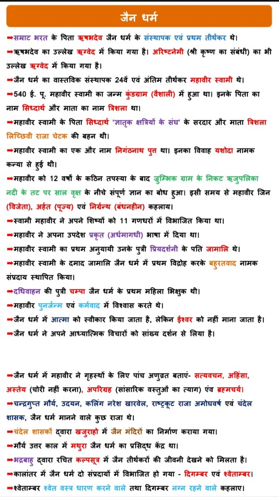
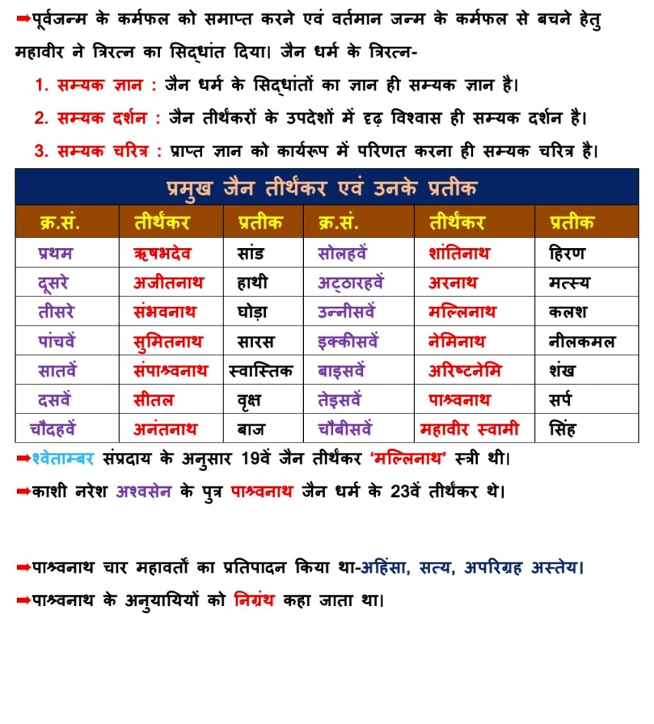
जैन धर्म श्रमण परम्परा से निकला है तथा इसके प्रवर्तक हैं २४ तीर्थंकर, जिनमें प्रथम तीर्थंकर भगवान ऋषभदेव (आदिनाथ) तथा अन्तिम तीर्थंकर महावीर स्वामी हैं। जैन धर्म की अत्यन्त प्राचीनता सिद्ध करने वाले अनेक उल्लेख साहित्य और विशेषकर पौराणिक साहित्यो में प्रचुर मात्रा में हैं। श्वेतांबर व दिगम्बर जैन पन्थ के दो सम्प्रदाय हैं, तथा इनके ग्रन्थ समयसार व तत्वार्थ सूत्र हैं। जैनों के प्रार्थना स्थल, जिनालय या मन्दिर कहलाते हैं।[1] कार्य करती है
जैन ध्वज ‘जिन परम्परा’ का अर्थ है – ‘जिन द्वारा प्रवर्तित दर्शन’। जो ‘जिन’ के अनुयायी हों उन्हें ‘जैन’ कहते हैं। ‘जिन’ शब्द बना है संस्कृत के ‘जि’ धातु से। ‘जि’ माने – जीतना। ‘जिन’ माने जीतने वाला। जिन्होंने अपने मन को जीत लिया, अपनी तन मन वाणी को जीत लिया और विशिष्ट आत्मज्ञान को पाकर सर्वज्ञ या पूर्णज्ञान प्राप्त किया उन आप्त पुरुष को जिनेन्द्र या जिन कहा जाता है’। जैन धर्म अर्थात ‘जिन’ भगवान् का धर्म।
अहिंसा जैन धर्म का मूल सिद्धान्त है। इसे बड़ी सख्ती से पालन किया जाता है खानपान आचार नियम मे विशेष रुप से देखा जा सकता है। जैन दर्शन में कण-कण स्वतंत्र है इस सॄष्टि का या किसी जीव का कोई कर्ताधर्ता नही है। सभी जीव अपने अपने कर्मों का फल भोगते है। जैन दर्शन में भगवान न कर्ता और न ही भोक्ता माने जाते हैं। जैन दर्शन मे सृष्टिकर्ता को कोई स्थान नहीं दिया गया है। जैन धर्म में अनेक शासन देवी-देवता हैं पर उनकी आराधना को कोई विशेष महत्व नहीं दिया जाता। जैन धर्म में तीर्थंकरों जिन्हें जिनदेव, जिनेन्द्र या वीतराग भगवान कहा जाता है इनकी आराधना का ही विशेष महत्व है। इन्हीं तीर्थंकरों का अनुसरण कर आत्मबोध, ज्ञान और तन और मन पर विजय पाने का प्रयास किया जाता है।
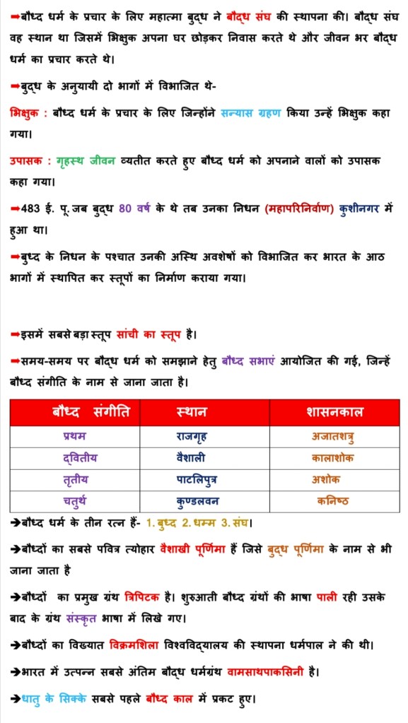
Buddhism is an ancient Indian religion, which arose in and around the ancient Kingdom of Magadha (now in Bihar, India), and is based on the teachings of Gautama Buddha[note 1] who was deemed a “Buddha” (“Awakened One”[3]), although Buddhist doctrine holds that there were other Buddhas before him. Buddhism spread outside of Magadha starting in the Buddha’s lifetime.
The Great Stupa at Sanchi, located in Sanchi, Madhya Pradesh, is a Buddhist shrine in India.
The Mahabodhi Temple, a UNESCO World Heritage Site, is one of the four holy sites related to the life of the Buddha, and particularly to the attainment of Enlightenment. The first temple was built by the Indian Emperor Ashoka in the 3rd century BC, and the present temple dates from the 5th century or 6th century AD. It is one of the earliest Buddhist temples built entirely in brick, still standing in India, from the late Gupta period.[1]
Rock-cut Buddha Statue at Bojjanakonda near Anakapalle of Visakhapatnam, Andhra Pradesh.
Ancient Buddhist monasteries near Dhamekh Stupa Monument Site in Sarnath.
Devotees performing puja at one of the Buddhist Caves in Ellora. During the reign of the Mauryan Emperor Ashoka, the Buddhist community split into two branches: the Mahāsāṃghika and the Sthaviravāda, each of which spread throughout India and split into numerous sub-sects.[4] In modern times, two major branches of Buddhism exist: the Theravada in Sri Lanka and Southeast Asia, and the Mahayana throughout the Himalayas and East Asia. The Buddhist tradition of Vajrayana is sometimes classified as a part of Mahayana Buddhism, but some scholars consider it to be a different branch altogether.[5]
The practice of Buddhism lost influence in India around the 7th century CE, after the collapse of the Gupta Empire. The last large state to support Buddhism—the Pala Empire—fell in the 12th century. By the end of the 12th century, Buddhism had largely disappeared from India with the exception of the Himalayan region and isolated remnants in parts of south India. However, since the 19th century, modern revivals of Buddhism have included the Maha Bodhi Society, the Vipassana movement, and the Dalit Buddhist movement spearheaded by B. R. Ambedkar. There has also been a growth in Tibetan Buddhism with the arrival of the Tibetan diaspora and the Tibetan government in exile in India, following the Chinese annexation of Tibet in 1950. According to the 2011 Census there are 8.4 million Buddhists in India (0.70% of the total population).
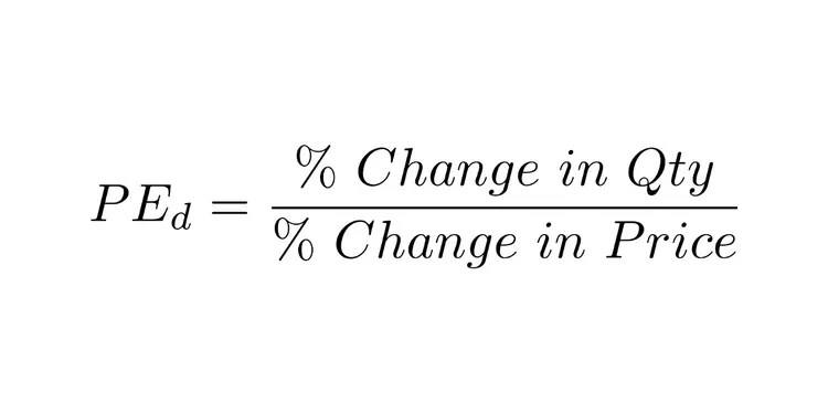
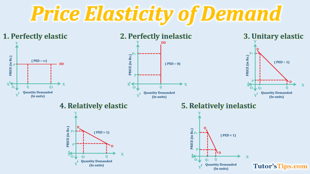
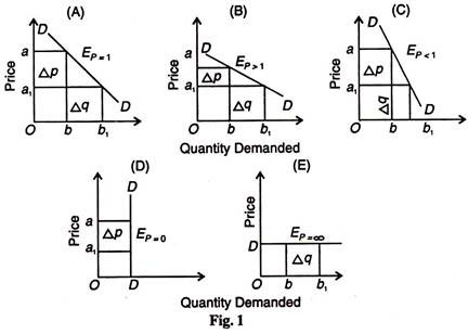
Elasticity of demand refers to the shift in demand for an item or service when a change occurs in one of the variables that buyers consider as part of their purchase decisions. It’s a relationship between demand and another variable, such as price, availability of substitutes, advertising pressure and customer income.FormulaFormula e_{(p)}=\frac{dQ/Q}{dP/P} https://youtube.com/@Bibekkumarsahu12?si=EGLTAuSfGYJzziWG
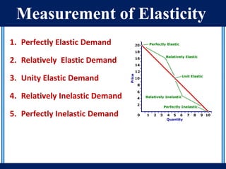
How Is Elasticity Measured?
Elasticity is measured by the ratio of two percentages: the percentage change in quantity demanded divided by the percentage change in price.
if �/� is constant.[13][14] There does exist a nonlinear shape of demand curve along which the elasticity is constant: �=��1/�, where � is a shift constant and � is the elasticity.
Second, percentage changes are not symmetric; instead, the percentage change between any two values depends on which one is chosen as the starting value and which as the ending value. For example, suppose that when the price rises from $10 to $16, the quantity falls from 100 units to 80. This is a price increase of 60% and a quantity decline of 20%, an elasticity of (−20%)/(+60%)≈−0.33 for that part of the demand curve. If the price falls from $16 to $10 and the quantity rises from 80 units to 100, however, the price decline is 37.5% and the quantity gain is 25%, an elasticity of (+25%)/(−37.5%)=−0.67 for the same part of the curve. This is an example of the index number problem.[15][16]
Two refinements of the definition of elasticity are used to deal with these shortcomings of the basic elasticity formula: arc elasticity and point elasticity.
Arc elasticity was introduced very early on by Hugh Dalton. It is very similar to an ordinary elasticity problem, but it adds in the index number problem. Arc Elasticity is a second solution to the asymmetry problem of having an elasticity dependent on which of the two given points on a demand curve is chosen as the “original” point will and which as the “new” one is to compute the percentage change in P and Q relative to the average of the two prices and the average of the two quantities, rather than just the change relative to one point or the other. Loosely speaking, this gives an “average” elasticity for the section of the actual demand curve—i.e., the arc of the curve—between the two points. As a result, this measure is known as the arc elasticity, in this case with respect to the price of the good. The arc elasticity is defined mathematically as:[16][17][18]��=(�1+�22)(��1+��22)×Δ��Δ�=�1+�2��1+��2×Δ��Δ�
This method for computing the price elasticity is also known as the “midpoints formula”, because the average price and average quantity are the coordinates of the midpoint of the straight line between the two given points.[15][18] This formula is an application of the midpoint method. However, because this formula implicitly assumes the section of the demand curve between those points is linear, the greater the curvature of the actual demand curve is over that range, the worse this approximation of its elasticity will be.[17][19]
The point elasticity of demand method is used to determine change in demand within the same demand curve, basically a very small amount of change in demand is measured through point elasticity. One way to avoid the accuracy problem described above is to minimize the difference between the starting and ending prices and quantities. This is the approach taken in the definition of point elasticity, which uses differential calculus to calculate the elasticity for an infinitesimal change in price and quantity at any given point on the demand curve:[20]��=d��d����
In other words, it is equal to the absolute value of the first derivative of quantity with respect to price d��d� multiplied by the point’s price (P) divided by its quantity (Qd).[21] However, the point elasticity can be computed only if the formula for the demand function, ��=�(�), is known so its derivative with respect to price, ���/��, can be determined.
In terms of partial-differential calculus, point elasticity of demand can be defined as follows:[22] let �(�,�) be the demand of goods �1,�2,…,�� as a function of parameters price and wealth, and let �ℓ(�,�) be the demand for good ℓ. The elasticity of demand for good �ℓ(�,�) with respect to price �� is��ℓ,��=∂�ℓ(�,�)∂��⋅���ℓ(�,�)=∂log�ℓ(�,�)∂log��
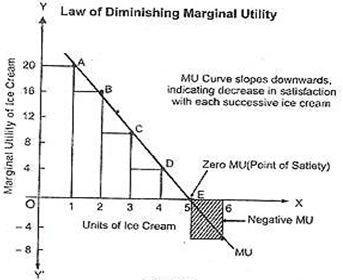
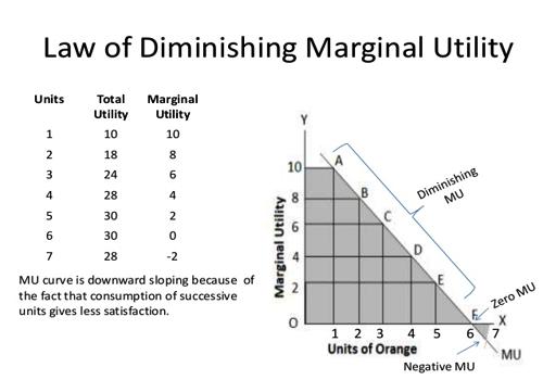
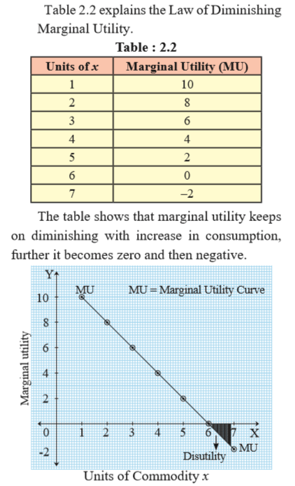
The law of diminishing marginal utility explains that as a person consumes an item or a product, the satisfaction or utility they derive from the product wanes as they consume more and more of that product. For example, an individual might buy a certain type of chocolate for a while. Soon, they may buy less and choose another type of chocolate or buy cookies instead because the satisfaction they were initially getting from the chocolate is diminishing.
In economics, the law of diminishing marginal utility states that the marginal utility of a good or service declines as more of it is consumed by an individual. Economic actors receive less and less satisfaction from consuming incremental amounts of a good.
KEY TAKEAWAYS
The law of diminishing marginal utility explains that as a person consumes more of an item or product, the satisfaction (utility) they derive from the product wanes.
Demand curves are downward sloping in microeconomic models since each additional unit of a good or service is put toward a less valuable use.
Salespeople often use different methodologies of soliciting sales as different customers have different reasons for buying a single quantity of an item.
Marketers use the law of diminishing marginal utility because they want to keep marginal utility high for products that they sell.
There are several laws of diminishing marginal units, each of which is different but tangentially related across the life cycle of a product.
Understanding the Law of Diminishing Marginal Utility
Whenever an individual interacts or consumes an economic good, that individual acts in a way that demonstrates the order in which they value the use of that good. Thus, the first unit that is consumed satisfies the consumer’s greatest need. The second unit results in a lesser amount of satisfaction, and so on.
null
For example, consider an individual on a deserted island who finds a case of bottled water that washes ashore. That person might drink the first bottle indicating that satisfying their thirst was the most important use of the water. The individual might bathe themselves with the second bottle, or they might decide to save it for later.
If they save it for later, this indicates that the person values the future use of the water more than bathing today, but still less than the immediate quenching of their thirst. This is called ordinal time preference. This concept helps explain savings and investing versus current consumption and spending.
The example above also helps to explain why demand curves are downward sloping in microeconomic models since each additional unit of a good or service is put toward a less valuable use.
Consumption of a good often begins with an increasing marginal utility for every good consumed followed by decreasing marginal utility for later units consumed.
Diminishing Marginal Utility Examples
The law of diminishing marginal utility is not specific to any industry. Its broad concept relates to different sector in different ways. In general, it is statistically proved that consumers exert more caution and attention when faced with higher utility propositions.1 Here are some ways diminishing marginal utility influences processes along a business process.
Sales
The technique of selling goods dramatically changes depending on the consumer’s current marginal utility potential. Consider a salesperson who is selling you your first cellphone. With your marginal utility very high with any working cellphone, the sale is easy. However, if you already own a cellphone, the tactics used by the salesperson (e.g., suggesting a different phone for work, suggesting a backup phone, suggesting upgrading your existing model) will differ.
Though not directly linked to the saying “read the room,” the concept of diminishing marginal utility is very relatable, as not every client will associate the same utility with a given product. When offered a single free peanut-butter-and-jelly sandwich, for example, some consumers (including those allergic to peanut butter) may have negative utility while most people will have positive marginal utility .
Manufacturing/Inventory Management
Companies must be mindful of the law of diminishing marginal utility when planning future production schedules. They can’t always rely on historical manufacturing levels, as changes in consumer demand will impact the number of goods needed.
This concept is especially important for companies that carry inventory. The law of diminishing marginal utility can produce a very steep drop-off. Again, consider the use of cellphones. Many people only need one; there is an incredibly large jump in utility from owning zero cellphones to owning one cellphone. Should a market become quickly saturated with people who all own cellphones, a company may be stuck holding inventory.
Marketing
Marketers use the law of diminishing marginal utility because they want to keep marginal utility high for the products that they sell. A product is consumed because it provides satisfaction, but too much of a product might mean that the marginal utility reaches zero because consumers have had enough of a product and are satiated. Of course, marginal utility depends on the consumer and the product being consumed.
This is an important concept for companies that have a diverse product mix. Imagine your favorite coffee shop. If the shop only marketed a single product, consumers would likely grow tired of that product; its marginal utility would diminish. Marketing professionals must juggle piquing demand for a variety of products to keep consumers interested in numerous products.
Some units may have zero marginal utility for the second unit consumed. For example, if you already own a copy of a magazine, there’s very little to no utility in owning a second copy. In these situations, the marginal utility has decreased 100% between units.
Diminishing Marginal Utility vs. Other Measurements
The law of diminishing marginal utility should not be confused with other laws of diminishing marginal units:
Diminishing marginal utility focuses on the consumer aspect and the decreasing nature of demand over time.
The law of diminishing marginal productivity states that the efficiency gained on slight process improvements may yield incremental benefits for additional units manufactured. An example of diminishing marginal product is labor costs to manufacture a car. It is more profitable to lay off 10% of the manufacturing staff, and the manufacturing line may make do with the remaining resources for the first few vehicles. However, after a while, the marginal manufacturing benefit decreases due to staff shortages.
The law of diminishing marginal revenue states that once maximum efficiency is reached, the amount of profit earned per unit will decrease. This can be due to a saturated nature of demand (i.e., diminishing marginal utility for consumers) or escalating production costs (i.e., diminishing marginal product for production).
Though all three laws are different, each carries with it concepts of economies of scale and is interrelated in the scope of the entire life cycle of a product.
What Is Meant By Marginal Utility?
Marginal utility is the benefit a consumer receives by consuming one additional unit. The benefit you receive for consuming every additional unit will be different, and the law of diminishing marginal utility states the benefit will eventually begin to decrease. The first slice of pizza you eat may be delicious, but the 15th slice may be a little painful.
What Is the Importance of the Law of Diminishing Marginal Utility?
The law of diminishing marginal utility dictates many aspects of how a company operates. A company must adjust how many goods it carries in inventory, as well as its sales tactics, because of the law. In addition, a company’s marketing strategy often revolves around balancing the marginal utility across product lines.
Can Marginal Utility Be Zero?
Yes, marginal utility not only can be zero but it can drop to below zero. Consider a summer barbeque. If you haven’t had breakfast yet, that first hot dog will be delicious and the second one won’t be bad either. After a while, you’ll become averse to eating hot dogs and may even get sick (have negative utility) if you continue to eat more.
The Bottom Line
There are exceptions to the law of diminishing marginal utility. For example, the law does not hold true in the case of collectors, who might be equally excited (or even more so) about buying their tenth rare coin as their first. Still, the law of diminishing marginal utility helps explain why consumers are generally less and less satisfied with each additional product.
The law of diminishing marginal utility states that as consumption increases, the marginal utility derived from each additional unit declines. Learn more.
Diminishing marginal utility refers to the phenomenon that each additional unit of gain leads to an ever-smaller increase in subjective value. For example, three bites of candy are better than two bites, but the twentieth bite does not add much to the experience beyond the nineteenth (and could even make it worse).


 Formula